

Linkage Framework: Human Activities - Pressures - Ecosystem Components
📌 About this Module 'Framework Hierarchy Viewer'
This module helps users explore the selected linkage framework, visualizing the relationships between Human Activities, Pressures, and Ecosystem Components.
The chord diagram below offers a visual representation of the connectivity between these elements, as defined by the chosen linkage framework. Frameworks may align with policy instruments such as the EU Marine Strategy Framework Directive (MSFD).
⚠️ Note: The chord plot below is designed solely for Illustration purposes. It summarizes the complex connections but does not show detailed data gaps.
For exploring the selcted framework, scroll down for an interactive table view or to the next tab: 'Linkage Visualization' to visualize the linkage framework based on your case study
Linkage Framework: Human Activities - Pressures - Ecosystem Components
This chord diagram visualizes how activities are connected to ecosystem components through pressures.
Hierarchical View of Activity-Pressure Linkages
How to Explore the Linkage Hierarchy
This interactive table presents the framework structured as a nested hierarchy, allowing you to navigate through the relationships between human activities and environmental pressures.
- Activity Groups: Broad categories grouping similar human uses or sectors (e.g., Fishing, Transport).
- Activities: Specific human activities within each group.
- Pressure Groups: General categories of pressures exerted by the activities.
- Pressures: Specific environmental pressures impacting ecosystem components.
Navigation Tips:
- Click the + icon next to each Activity Group to expand and see its associated activities.
- Click the + icon next to an Activity to view the detailed pressures it generates.
- Use the filter or search box to quickly find specific activities or pressures.
- Collapse groups as needed to simplify your view while exploring large datasets.
This view helps you visualize the full linkage network between human activities and ecosystem pressures in a clear, expandable format.
Framework Hierarchy Flow
Use this expandable table below to explore or download the detailed linkages:
Download Nested CSV📌 About this Module 'Linkage Visualization'
This module allows you to explore and visualize the connections between Activities, Pressures, and Ecosystem Components (ECs) for your selected data (e.g. spatial layers). The goal is to help you understand potential interactions and identify data gaps before proceeding to the Cumulative Effects Assessment (CEA) analysis.
Select the available layers for your study area. The Sankey plot below provides a visual representation of the linkages present in your data.
⚠️ The interactive tables below the Sankey chart are designed to assist you in reviewing potential data gaps or missing connections.
These tables serve as guidance and reference points, helping you consider additional data or linkages that may be relevant for your case study before running the full CEA model.
Interactive Sankey (Plotly)
Selected linkages: only shows links that exist in your current selection. Full framework: shows all framework links; colored thick links = covered by your selected pressure layers; thin light-gray = gaps.
Tip: hover to see source → target links and counts. Links are colored by Pressure.
The plot above is color-coded to show the pressures with direct linkages to the activities and ecosystem components selected in the side panel. If an activity or pressure is missing from the plot, it indicates there are no direct linkages to other layers within the selected linkage framework. Refer to the tables below for more detailed information.
Missing pressures for selected Ecosystem components
IMPORTANT: Below are various pressures that may affect the selected ecosystem components, which you may wish to consider adding to your CEA analysis or considering as gaps in your CEA analysis and conclusions.
Download Missing Data TableActivities with no connection to selected Pressures
The table below lists activities that do not have an explicit link to the selected pressures based on the linkage framework. For each of these activities, their corresponding activity group is shown, along with the pressures associated with that group and their dispersive (D) or non-dispersive (ND) classification.
A non-dispersive (ND) pressure means that the spatial footprint of the human activity can be directly used as the spatial extent of the pressure in your CEA analysis. In contrast, a dispersive (D) pressure requires additional modeling (e.g., Gaussian dispersion, buffers, or hydrodynamic models) to estimate the actual footprint of the pressure. This information helps guide you in determining which pressures can be mapped directly and which ones need further spatial modeling.
Use this table to review potential pressures exerted by the disconnected activities that may not be explicitly captured in your current selection but are part of the linkage framework.
IMPORTANT: For the selected activities below, consider mapping their associated pressure layers to continue your CEA analysis. For non-dispersive (ND) pressures, refer to the table below to identify which pressures are classified as ND. You can then use the 'Mapping - non-dispersive (ND) Pressure Layers' Tab to spatially generate these pressure layers based on your activity data.
Download Disconnected Activities TableMissing activities for selected Pressures
IMPORTANT: Below are various activities (columns) that contribute to your selected pressures under the selected linkage framework. 1) you may want to consider adding to your CEA analysis, OR 2) may already be included in your pressure layer, OR 3) you may want to consider as gaps in your CEA analysis and conclusions.
Download Missing Activities Table
Developed by Meeresnutzungskonzepte gruppe / Marine spatial management group
Juan Camilo Cubillos
Contact email: juan.cubillos@thuenen.de
version: 1.5 (09.05.20)
📌 About this Module — Assessment Gaps
This section gives a simple, transparent metric of how complete your CEA is, based on the linkage framework and the layers you’ve selected.
What the gauge shows
- Completeness (LCI_overall) [0–1]: 1 = most expected linkages are covered; 0 = very little coverage.
- Uncertainty = 1 − Completeness: the share of expected linkages not covered by your data.
How the score is built
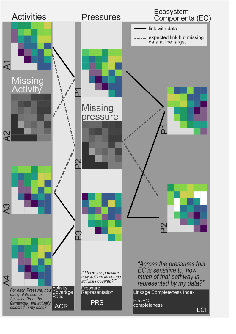
- Activity Coverage Ratio (ACR) : for each Pressure, ACR(p) = (# selected Activities generating p) / (all Activities generating p in the framework) .
- Pressure Representation (PRS) : for each Pressure, PRS(p) = Presence_of_layer(p) × ACR(p) .
-
Per-EC completeness (LCI)
: combine PRS with sensitivity
S(p,EC)via LCI(EC) = Σ[S×PRS] / Σ[S] . - Overall completeness : sensitivity-weighted average of LCI across your selected ECs.
- Top Pressure Gaps : priority = (1 − PRS) × relative sensitivity mass — where adding data would most reduce uncertainty.
Sensitivity options (S)
- Binary (default): any ‘x’ in the framework = 1 (linked); blank = 0.
- Manual: edit a pre-filled matrix (0–1) inside this tab.
- Upload: download the template (names pre-matched), fill values (0–1), and upload.
Note: Sensitivities are context-dependent. Literature can guide you, but local conditions often justify adjustments.
Completeness reflects how much of the expected impact chains are covered by your selected data. See the description on the left or the Help Tab for details.
Contribution breakdown (per ecosystem component)
Top Pressure Gaps
- Priority (0–1): bigger payoff from adding or improving this pressure’s data. Computed as Gap size × Importance .
- Gap size (0–1): how under-represented this pressure is now. 1 = pressure missing (no layer or no linked activities); 0 = fully represented.
- Importance (0–1): how relevant the pressure is for your selected ECs, based on their sensitivities (scaled relative to the most sensitive pressure).
- Representation (PRS): current coverage of the pressure (presence × activity coverage).
Why Priority can be 0: either the pressure is already fully covered (Gap size = 0) or none of your selected ECs are sensitive to it (Importance = 0).
Ecosystems Most Affected
Sensitivity matrix (optional)
Choose how to provide P→EC sensitivities S(p,EC) used by the completeness gauge.
Template preview (for reference):
Debug (dev only)
📌 About this Module 'Non-Dispersive (ND) Pressure Mapping'
This module allows users to map spatial footprints of non-dispersive (ND) pressures derived from human activities.
ND pressures represent those that are spatially confined to the activity footprint, such as localized physical disturbance or habitat loss.
⚠️ Careful consideration is required when mapping ND pressures. Users should:
- Refer to scientific studies, technical reports, or guidance documents when determining if an activity generates ND or Dispersive (D) pressures.
- Consult the 'Activities with no connection to selected Pressures' in the Linkage Visualization Tab for possible 'ND/D Pressures' for your case study, for suggestions based on previous publications
- Avoid rasterizing activities that inherently produce dispersive pressures (e.g., nutrient runoff, noise propagation, contaminant plumes).
The tool enables rasterizing uploaded activity layers (points, lines, polygons) into a user-defined grid, allowing generation of ND pressure layers suitable for further analysis.
Output GeoTIFFs represent the intensity or presence of ND pressures within each grid cell.
🚀 Reminder: Buffer distances and aggregation types significantly influence the final raster layer. Ensure parameter choices reflect the ecological and spatial context of your assessment.
🚀🚀 Second Reminder: While this module allows you the visualizazion of raster layers, does not allow any manipulation of raster file, might lead to the app come crashing back to earth in the blink of an eye
1. Upload Activity Data
💾 Tip: For shapefiles, upload a single .zip containing .shp, .shx, .dbf, .prj files.
📌 NOTE: If uploading a Shapefile, select all related files (.shp, .shx, .dbf, .prj) together.Uploaded Layer Summary
2. Select the type of aggregation
3. ND Pressure output
⚠️ Preview map grid resolution is capped at 0.2° for computational performance. Higher grid resolution (e.g., 0.05°), will be applied to the GeoTIFF output
ND Pressure Layer (Grid Result)
Download ND Grid as GeoTIFF📌 About this Module 'Temporal Coverage Assessment'
This module helps you assess the temporal distribution of your available data, allowing you to identify potential mismatches, gaps, or inconsistencies that could impact the conclusions of your Cumulative Effects Assessment (CEA) analysis.
You can define the temporal scope for each dataset type (Activities, Pressures, Ecosystem Components) by adjusting the slider nodes below.
⚠️ The interactive plot visualizes the selected time frames, highlighting any potential temporal gaps or overlaps between human activities, pressures, and ecosystem components within your case study.
Proper temporal alignment is essential to ensure the robustness and relevance of your CEA results.
🚨 Important Consideration: While temporal gaps between pressures and ecosystem components may appear in the visualization, it is up to the user to evaluate their ecological significance.
For example, some pressures might have long-lasting impacts (e.g., seabed disturbance) while others may cause short-term effects (e.g., phytoplankton bloom suppression).
Always assess if these temporal mismatches could affect your conclusions or require further attention in your analysis.
Activities
Pressures
Ecosystem Components
The table below shows the temporal overlap between pressures and Ecosystem components. Consider how temporal explict your non- or poorly overlaping layers can affect your conlusions from CEA
🚨 Important Consideration: The table below might shows pairing of all pressures to EC in terms of temporal overlap however in the current app version does not account for actual linkages from the selected Linkage framework. Please consider this and review.
Developed by Meeresnutzungskonzepte gruppe / Marine spatial management group
Juan Camilo Cubillos
Contact email: juan.cubillos@thuenen.de
version: 1.5 (09.05.20)
Purpose of the App
The Pressure2Eco Shiny app has been designed to assist users in preparing for a Cumulative Effects Assessment (CEA). It allows users to evaluate the linkages between spatially available layers and their connections to activities, pressures, and ecosystem components. Additionally, the app helps identify potential gaps or missing data, assess the quality of linkages, and address possible temporal mismatches in the data before conducting the CEA analysis. It provides support using three widely recognized linkage frameworks, ensuring a comprehensive evaluation of the data prior to further analysis.
Understanding the Linkage Frameworks
Here you can find detailed explanations about each linkage framework, their sources, and important considerations. These linkage frameqoerk provide a conceptual map of linkage chains between the main elements of a CEA: Human activities, Pressures and Ecosystem components (e.g. Habitats, Species or Taxonomical groups.)
1. Linkage Frameworks
The three main linkage frameworks supported are ODEMM, SCAIRM, and HELCOM. Each framework links activities, pressures, and ecosystem components differently based on specific environmental and human impact models.
The source data for these Linkages frameworks comes from the following sources:
- MSFD: Marine Strategy Framework Directive; European Commission, 2022. MSFD CIS Guidance Document No. 19, Article 8 MSFD, May 2022
- SCAIRM: Spatial Cumulative Assessment of Impact Risk for Management; Piet et al. 2023. Source: SCAIRM Coolbook and
- ODEMM: Options for Delivering Ecosystem-Based Marine Management. Source: Derived from ODEMM WP 4
- HELCOM: Baltic Marine Environment Protection Commission (Helsinki Commission - HELCOM). Source:
2. Plot Explanation
The interactive Sankey diagram in the 'Linkage Visualization' tab shows how your selected Activities connect to Pressures, and how those Pressures connect to Ecosystem Components (ECs). Link thickness reflects the number of reported linkages within the selected framework and your current selections.
Tips for interpreting the Sankey:
- Missing data: If an expected pressure or EC is absent, it may indicate a data gap or an unselected layer.
- Disconnected activities: Activities with no links to selected pressures won’t appear on the left. Check the 'Activities with no connection to selected Pressures' table.
- Missing activities for pressures: If a pressure is present but some of its source activities are unselected, those contributions won’t be shown.
- Sensitivity is not shown in the Sankey; it’s handled in the Gaps tab via the sensitivity matrix.
3. Assessment Gaps
📌 How the 'Assessment Gaps' score is computed (step by step)
1) Activity Coverage Ratio (ACR) — per Pressure
Plain question: “For this Pressure, how many of its source Activities (in the framework) are actually selected in my case?”
Equation:
ACR(p) = selected_acts(p) / all_acts(p)
∈ [0,1]
2) Pressure presence (Ip) — per Pressure
Plain question: “Do I have this pressure layer?”
Rule:
Ip(p) = 1
if the pressure layer is present;
0
if it is missing.
3) Pressure Representation Score (PRS) — per Pressure
Plain question: “If I have this pressure, how well are its source activities covered?”
Equation:
PRS(p) = Ip(p) × ACR(p)
∈ [0,1]
4) Sensitivity matrix S(p, EC) — Pressure → Ecosystem Component
The sensitivity
S(p, EC)
describes how strongly a Pressure (p) affects an Ecosystem Component (EC).
You can use the default binary values from the framework (x = 1, blank = 0),
edit them manually, or upload your own numeric values in [0,1].
5) Per-EC Linkage Completeness (LCI) — per EC
Plain question: “Across the pressures this EC is sensitive to, how much of that pathway is represented by my data?”
Equation:
LCI(EC) = ( Σ_p [ S(p,EC) × PRS(p) ] ) / ( Σ_p S(p,EC) )
(if the denominator is 0, we use a conservative default in the app).
6) Overall completeness (the gauge) — across selected ECs
Plain question: “Across all selected ECs, how complete is my assessment, giving more weight to ECs with more relevant linkages?”
Equation:
LCI_overall = ( Σ_EC [ W(EC) × LCI(EC) ] ) / ( Σ_EC W(EC) )
, where
W(EC) = Σ_p S(p,EC)
.
Uncertainty:
Uncertainty = 1 − LCI_overall
7) Top Pressure Gaps (priority) — per Pressure
Plain question: “Which pressures, if added or improved, would most reduce uncertainty for my ECs?”
Equation:
PGP(p) = (1 − PRS(p)) × ( Σ_EC S(p,EC) / max_p Σ_EC S(p,EC) )
— higher values indicate higher priority to address.
Optional diagnostic: Activity Representation Score (ARS) — per Activity
Plain question: “For this Activity, how well are its expected pressures represented by my current pressure layers?”
Example definition (diagnostic only):
ARS(a) = mean_{p ∈ P(a)} PRS(p)
— ARS helps explain gaps but does not enter the gauge.
How to increase the gauge
-
Select missing pressure layers:
raises
Ip→ raisesPRS. -
Select more relevant activities:
raises
ACRfor their pressures → raisesPRS. -
Refine sensitivities:
adjust
S(p,EC)to reflect local knowledge; this changes how completeness is averaged across linkages and ECs.
4. Spatial ND Pressure Layer
This section helps you generate spatial layers for pressures classified as Non-Dispersive (ND). ND pressures are those where the spatial extent of the pressure is equivalent to the footprint of the activity causing it, meaning no further dispersal modeling is needed.
Examples of ND pressures include:
- Seabed abrasion from bottom trawling
- Physical habitat loss due to construction or dredging
- Localized sediment resuspension
The tool allows you to:
- Upload your spatial activity data (points, lines, polygons, or raster)
- Preview your data on a map
- Define a spatial grid resolution (e.g., 0.05°)
- Choose an aggregation method:
- Presence/Absence - 1 if activity is present, 0 otherwise
- Count Points - Number of points in each grid cell
- Count Geometries - Number of lines or polygons intersecting each grid cell
- Optionally apply a buffer to expand the activity's spatial influence
Applying a buffer is useful when the impact extends beyond the activity footprint depending on literature or expert knowledge. For example, dredging operations may affect adjacent areas due to sediment plumes if this values are known for your area of study or literature to support the buffer.
The output is a gridded pressure layer representing either presence/absence or intensity (counts), ready for download as a GeoTIFF for further analysis.
💡 Important Note: For Non-Dispersive pressures, using the activity footprint is appropriate for mapping the spatial extent of the pressure prior to your Cumulative Effects Assessment (CEA).
For detailed methodology and examples, refer to: Goodsir et al., 2015 - A spatially resolved pressure-based approach
5. Temporal Coverage and Gaps
The temporal coverage sliders allow you to specify the years of available data for each Activity, Pressure, and Ecosystem Component. It is important to note that the temporal data may have gaps, which can affect the conclusions of your CEA.
For example:
- If an activity is only available in certain years, it may not accurately represent current or future conditions.
- Disparities in the temporal coverage between Activities, Pressures, and Ecosystem Components may affect the linkage interpretation.
- A temporal gap in one of the layers could lead to missing or incomplete connections, which should be addressed before proceeding with a CEA.
In general, you should always verify that the temporal coverage of all relevant layers is aligned and that the data gaps are understood before conducting a CEA.
5.1 Temporal Metrics Table: Explanation
The table below presents the temporal overlap between pressure layers and ecosystem components. It helps assess the temporal alignment of these layers, which is important for understanding the timing and interactions between environmental pressures and ecosystem dynamics. The key metrics displayed in the table are:
- *Overlap Percent*: This metric represents the percentage of time that a pressure layer and an ecosystem layer overlap. It is calculated by finding the number of overlapping years between the pressure and ecosystem layers and dividing this by the total number of years in the ecosystem layer. This value is expressed as a percentage.
- *Lead Gap*: The lead gap measures the amount of time that the ecosystem layer starts after the pressure layer ends. If the ecosystem layer begins after the pressure layer has already ended, the lead gap is the difference in years between the end of the pressure layer and the start of the ecosystem layer. If the ecosystem layer starts during or before the pressure layer ends, the lead gap is 0.
- *Lag Gap*: The lag gap measures the amount of time that the pressure layer starts after the ecosystem layer ends. If the pressure layer begins after the ecosystem layer ends, the lag gap is the difference in years between the start of the pressure layer and the end of the ecosystem layer. If the pressure layer starts before or during the ecosystem layer ends, the lag gap is 0.
The metrics presented in the table allow for evaluating how well the pressures align with the ecosystems over time. A high overlap percentage indicates strong temporal alignment, while a larger lead or lag gap indicates misalignment between the pressure and ecosystem layers. Understanding these temporal relationships can inform conclusions from causal effect analysis (CEA), as non-overlapping or poorly overlapping layers may lead to inaccurate interpretations or missed impacts.
Developed by:
Developed by Meeresnutzungskonzepte gruppe / Marine spatial management group
Juan Camilo Cubillos
Contact email: juan.cubillos@thuenen.de
version: 1.5 (09.05.20)
About This Application
The Pressure2Eco has been designed to support the workflow of Cumulative Effects Assessment (CEA) by allowing users to visualize linkages, idewntify data gaps, assess temporal coverage, and spatially map non-dispersive (ND) pressures prior to using other tools such as the GES4SEAS Toolbox.
Version History
- Version 1.1: Released March 2025 - Linkage visualization and identification of data gaps for your study.
- Version 1.2: Temporal coverage analysis added to assess spatial layer timelines and overlaps.
- Version 1.3: Framework Overview enhancements and addition of mapping tools for non-dispersive (ND) pressure layers.
- Version 1.4: Framework Hierarchy View Table functionality and adaptation of MSFD-SCAIRM.
- Version 1.5: Implementation of MSFD Framework based on the Guidance Document 19 for Article 8.
Contributions
This tool has been developed under the EU Horizon 2020 “GES4SEAS” project (Grant agreement ID: 101059877) and had contributions of:
- Juan Camilo Cubillos, Dr. Vanessa Stelzenmüller & Dr. Jennifer Rehren (Thünen Institute) - Conceptual design and R-shiny app architecture.
- Dr. Angel Borja, Dr. María C. Uyarra and Dr. Iratxe Menchaca (AZTI) – guidance on MSFD-2022 standardization and data harmonization.
- Dr. Gerjan Piet and Dr. Jacqueline Tamis (Wageningen University & Research) – guidance on SCAIRM and MSFD aligned SCAIRM linkage framework.
- Open-source community – for the R packages (sf, raster, ggalluvial, circlize, reactable, etc.) that are the beating heart and powerhouse of this Webapp.
Contact
For more information, feedback, or to report bugs, please contact:
Juan Camilo Cubillos
Email: juan.cubillos@thuenen.de
Marine Spatial Management Group, Thünen Institute
Version: 1.5